Abstract Derivatives Part 1

Cool Math Stuff
Author

Vaishnav Sudarshan

Published

November 23, 2025

Abstract
Answering the following questions - Why are matrices considered linear? How can differentiation also be interpreted as such?

Linear Operators

A linear operator \(L\) is just anything that satisfies \(L(ax+by)=aL(x)+bL(y)\), for constants \(a\) and \(b\), and where addition and multiplication are defined. In other words, it is additive, and you can pull out constants from the inside.

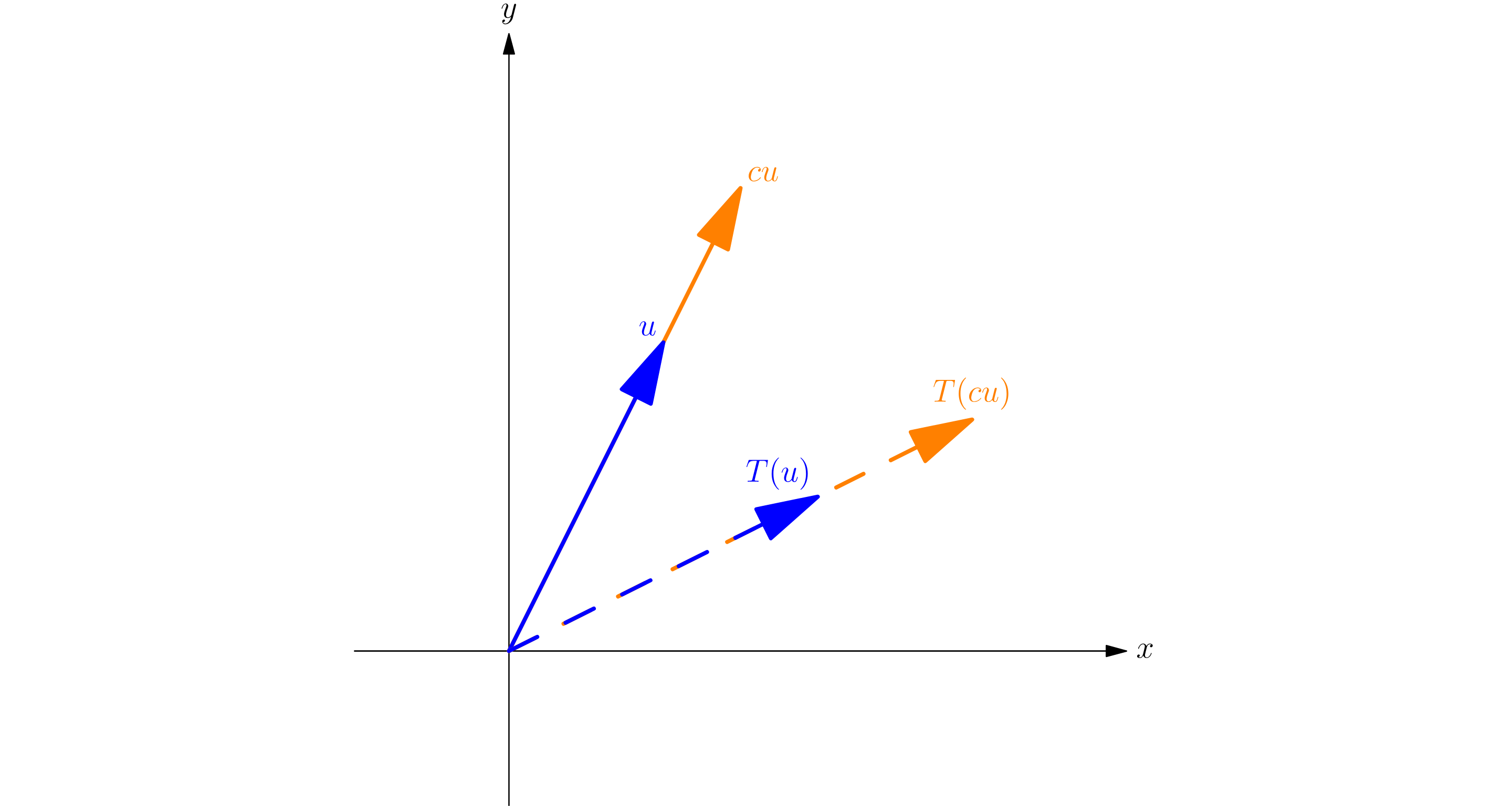
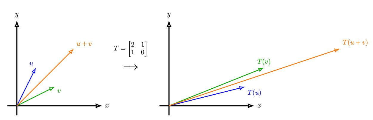
Matrices are where you probably saw this. If you transform a vector \(x\) by multiplying it with \(A\), do the same for a vector \(y\), and add the two new vectors, it’s the same as just adding them first and then transforming them. Also, if you scale \(x\) and \(y\) by some constants, it doesn’t matter if you did it before or after the transformation.

Diagram showing the constants rule of linear transformations

Diagram showing the constants rule of linear transformations

Diagram showing additivity of linear transformations

Diagram showing additivity of linear transformations

Derivatives As Linear Operators

Do you remember the sum and product rules of single-variable derivatives?

\(\frac{d}{dx} (af(x)) = a \frac{d}{dx} f(x)\) \(\frac{d}{dx} (f(x) + g(x)) = \frac{d}{dx} f(x) + \frac{d}{dx} g(x)\)

Wait, what??? Differentiation is also a linear operator on functions??? Now you realize how cool generalizing stuff is.

Hold on. Is \(y=mx+b\) linear on \(x\), for \(b \neq 0\)? The answer, surprisingly, is no. \(m(x_1+x_2)+b \neq (mx_1+b)+(mx_2+b)\). Linear, in this the context of this blog post, doesn’t necessarily mean the function is a line, but rather that the function behaves like a linear operator, which are typically different things. However, don’t think this form of function isn’t useful outside of 7th grade - when generalized to matrices, these can be very useful in AI.

Slight Tangent on Affine Transformations

Transformations of the form \(y=mx+b\) aren’t linear, but instead affine. Obviously not everything has to be a scalar, but instead can be about vectors and matrices where you have \(f(\vec{v}) = A \vec{v} + \vec{b}\) for some matrix \(A\). Where are affine transformations actually used?

A really common example is to get from one layer of a neural network to another, right before the activation function (more on that in the blog about neural networks). You multiply the vector of inputs in one layer by the matrix of weights and add to that the vector of biases to get the next layer pre-activation.

Making Derivatives More Abstract

For single variable functions, we have a scalar in and a scalar out (one input, one output). You could technically think of it as 1D vectors, as we’ll do soon, but it’s basically the same thing.

The main thing we want to emphasize here is that for the derivative, we write it as differentials (\(df = f'(x) dx\)) instead of \(\frac{df}{dx}\). In scalar functions, that works, but later on, it won’t make much sense to divide by a vector or a matrix.

Derivatives, however, aren’t just limited to acting on single-variables to be linear operators. Here are some other types of derivatives.

Multivariable Functions

For multivariable functions, we have many inputs in and one output out, where each input or output is a number. However, one interpretation of a vector is a list of numbers, so one could think of it as a vector in and a scalar out. What this means is that, for a 2D input space, \(f(\vec{x}) = f(x, y)\). For any point, or vector, on the 2D \(xy\) plane, there is a \(z\) coordinate corresponding to that, to form some sort of surface.

Again, what we basically just mean in this case is that a vector has two or more dimensions, and a scalar has just one. If we think of a list of numbers as a vector, then we can do vector operations on it, but if we think of a single number as a vector, doing vector operations on it wouldn’t make a difference.

As for the derivative? It’s a vector, known as the gradient! It is the vector of partial derivatives with respect to each variable. The gradient will always have the same “shape” as the input space, because it also represents the direction of steepest ascent. It’s written as \(\nabla f = [...\frac{\partial f}{\partial x_i}...]\), where \(x_i\) is each component in the input.

Slight Tangent on Gradient Descent

Why? Because think about this way: in differential form, we can write \(df = \Sigma {(\frac{\partial f}{\partial x_i} dx_i)}\). Oh, the sum of the corresponding products? Reminds me of dot product! We can write this as \(df = \nabla f \cdot \vec{dx}\). In terms of magnitudes, it can also be written as \(df = |\nabla f| |d\vec{x}| \cos(\theta)\). We can’t really do much with the given magnitudes to maximize \(df\).

At a particular input point \(\vec{x}\), the magnitude of \(\nabla f\) is going to be some constant when we’re dealing with anything but that input point and the function. Also, the magnitude of \(d\vec{x}\) can’t be dealt with because it’s an infinitesimal, not an actual number. So, the only thing we can do to maximize \(df\) is the \(\cos(\theta)\) term. The maximum of \(\cos(\theta)\) is \(1\), when \(\theta = 0^\circ\). So, if \(d\vec{x}\) is in the same direction as the gradient, the function increases the most.

Similarly, for \(df\) to be as low as possible, we want \(\cos(\theta)\) to be at its minimum (\(-1\)), which is when \(\theta = 180^\circ\), or when we move in the opposite direction as the gradient. Now, it is guaranteed that \(df \leq 0\), because we’re dealing with just magnitudes (always nonnegative) times \(-1\).

So, we can do some local linearization. If we have some random point \(\vec{x}, f(\vec{x})\), we can change \(\vec{x}\) by some small vector in the opposite direction of \(\nabla f\). Where do we get that small vector? First, we normalize \(-\nabla f\) by dividing by its magnitude to get a unit vector. Then, to scale it so that our local linearization approximation isn’t horrendous, we multiply this vector by a small scalar \(\mu\), known as the learning step. We subtract add this to the original \(\vec{x}\), and recalculate \(f(\vec{x})\).

For more on this, visit my blog on neural networks.

Vector-Valued Functions

What about a vector output for a scalar input? This could be represented as a parametric equation, and the derivative would also be a vector. An example of this is in physics, with velocity and acceleration, both as a function of time. See the diagram for these in circular motion.

Diagram showing the vector-valued functions of velocity and acceleration during circular motion

Diagram showing the vector-valued functions of velocity and acceleration during circular motion

To demonstrate where more abstract derivatives can be used in this case, we can use parametric equations. Let the counterclockwise angle above the horizontal of the particle moving in a circle be \(\theta\), and the radius be \(r\). From components, the direction of the position of the particle from the center is \([\cos(\theta), \sin(\theta)]\). Then, from geometry, since motion is perpendicular to the radius, the horizontal component of velocity (assuming constant speed \(v\)) is \(-v \sin(\theta)\), and the vertical component is \(v \cos(\theta)\). Given that \(\omega = d\theta/dt\) and \(v=\omega r\), try to prove for yourself that the centripetal acceleration must have magnitude \(\frac{v^2}{r}\) and point towards the center! The full solution is in my blog post about circular motion.

Vector Fields

At this point, we are exiting the more basic types of functions, and finally, matrices come into use here. You may recall that a vector field is a kind of function where for every point (vector) in space, there is an output which is a vector that moves that input somewhere else. As a result, what we can get by reiterating this process can be modeled for something like fluid flow. Maybe you’ve seen some of these diagrams before. Typically, since varying magnitudes get out of hand when drawn on paper, each point has a vector of a fixed length showing just direction, and the magnitudes are portrayed through color, where the “hotter” the color, the longer the magnitude is.

Diagram showing a vector field

Diagram showing a vector field

The diagram even looks intuitive. At each point, it tells you where to go next, and by how much. Even if you had no idea about what vector fields are, that’s literally what is looks like.

The derivative is a matrix called the Jacobian. Each row is basically the gradient with respect to the entire input from each component of the output.

If you think of it as looking at each component of the input, the Jacobian is also the derivative of the entire output with respect to each input.

So, if the input space is a vector in \(\mathbb{R}^n\) and the output space is a vector in \(\mathbb{R}^m\), the Jacobian is a matrix with dimensions \(m \times n\).

Now, the derivative can be written as \(d \vec{f} = J d \vec{x}\) for the Jacobian \(J\). Now, this looks like a proper matrix multiplication with no scalars involved apart from doing things component-wise.

One cool thing now is that if \(J\) is a constant matrix, the vector field is just a normal linear transformation of \(\vec{f}(\vec{x}) = J \vec{x}\), which is an interesting interpretation of linear transformations.

Conclusion

So far, what we’ve seen is just seeing pretty simple derivatives with a new interpretation. Stay tuned